PG Raster (continued)
I have a few more notes for working with PostGIS 2.0 raster types. I seem to have forgotten (and subsequently remembered) a few more things since my last work with these. One is:
Georeferencing properties
Make sure to use ST_SetGeoReference() to set all of the georeferencing properties of the raster. If you don’t, PostGIS will just quietly use pixel space in its stead, which is not right. I forgot to do this for the second raster that I loaded, and couldn’t figure out why an ST_Intersects() on the raster (all of BC) and the Peace boundaries (fully contained by BC) did not return true. Which leads me to the next point…
Y Scale
When setting the scale with something like this:
UPDATE bcsd SET rast = ST_SetScale(rast, 0.0625, 0.0625);
ignore what it says in the PostGIS book (page 391-ish) about having a negative y scale value. I think that that only applies for regular images. Also, when I set the yscale to be negative, the envelope of the raster of BC goes down south to like 35 degrees, which is obviously wrong. Although, for what it’s worth, QGIS’s (1.8.0) PostGIS raster plugin crashes when trying to load the raster with a positive y scale. But with a negative y scale (which is wrong anyways) QGIS will display the raster, but upside down. Suffice it to say, QGIS has a bit of work to do on these features and we probably won’t be able to utilize them for a few months at least.
Spatial indexes
Somehow on the first read, I missed the fact that you need to index the convex hull of the raster, rather than just the raster itself. So compute the index like so:
CREATE INDEX idx_bcsd_rast ON bcsd USING gist(ST_ConvexHull(rast));
With the indexes in place we can clip rasters to a polygon in a reasonable amount of time. I was able to clip the BCSD data to the Peace region (undecimated) in about 11 seconds. Not necessarily fast enough to run a web app off of, but it’s not slow either.
raster_test=> SELECT write_file(ST_AsGDALRaster(ST_Clip(rast, the_geom), 'GTiff'), 'blah.tiff') FROM basins INNER JOIN bcsd ON ST_Intersects(rast, the_geom);
 write_file
________________
 blah.tiff
 blah.tiff
(2 rows)

Time: 11397.841 ms
Although, that seems too slow… I wonder what happens if I limit it to one single band.
raster_test=> SELECT write_file(ST_AsGDALRaster(ST_Clip(rast, 1, the_geom), 'GTiff'), 'blah.tiff') FROM basins INNER JOIN bcsd ON ST_Intersects(rast, the_geom) WHERE rid=2;
 write_file
___________________
 blah.tiff
(1 row)

Time: 444.097 ms
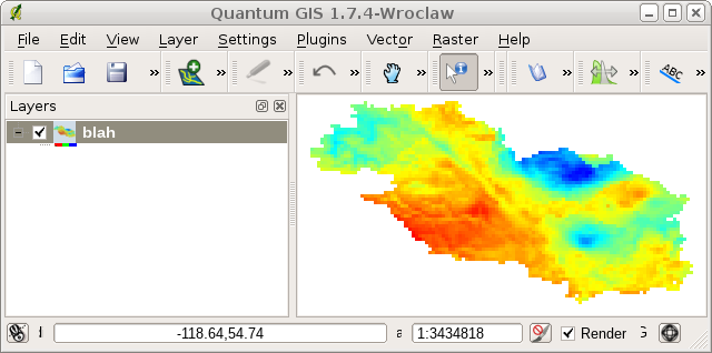
Ah ha! That’s fast enough to run a web app off of. I wonder why it reruns the clip operation on each band. I think that it has something to do with the nodata value… which incidentally doesn’t seem to be set for each band. I’ll have to experiment more with that. But anyways, after clipping and exporting to a geotiff, the image seems to come out in QGIS pretty nicely.
That’s all I have for now. More later.
blog comments powered by Disqus