Optimizing the Bias Correcting Constructed Analogues algorithm

Climate downscaling in a nutshell

When analyzing future climate change at PCIC, a large part of our job involves “downscaling” Global Climate Models (GCMs). This is forming statistical relationships between the spatially coarse-scale GCMs and fine scale topographic models and gridded observations. This is complex work and an area of active research and as such requires us to have a full “theme” (i.e. a division) dedicated to the task.

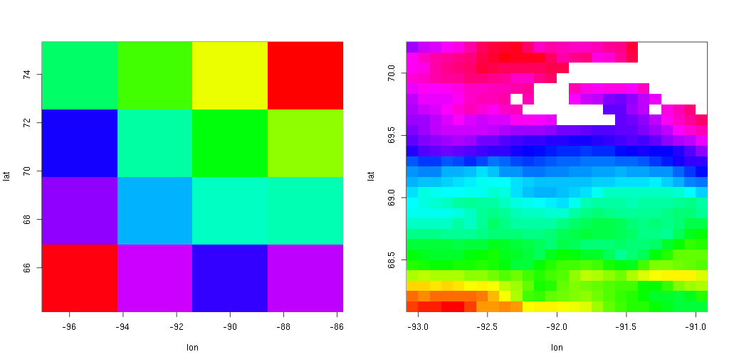GCM vs. downscaled output The middle four 100km resolution grid cells on the left are downscaled to 10km resolution on the right. Notice how many spatial patterns in the downscaled output are completely unrecognizable in the GCM. Downscaling adds lots and lots of value to GCM output.

The computational and storage costs of dowscaling are high, and so I have spent a fair amount of my time mitigating these costs by reducing the computational complexity. The Bias Correction Constructed Analogues (BCCA) algorithm is by far the most expensive, so I’ve spent a substantial amount of time on it.

What’s so expensive about BCCA? Let me try to explain.

What is Computational Complexity?

In Computer Science, we measure computational complexity of a particular task or algorithm as a function of the size of the input. This is referred to as big-O notation. For example, to find the minimum of $n$ numbers, one has to look at each and every one of them. Therefore the computational complexity of the function $min()$ is $O(n)$ . Sorting a list of unsorted numbers requires multiple passes over the $n$ input items, and depending on the algorithm, ranges from $O(n \ln{n})$ to $O(n^2)$ . Algorithms that compute the exact same result, can have vastly different computational complexities and this vastly different computational costs. For this reason, when optimizing programs, the biggest gains often come from rewriting the underlying algorithm.

The main purpose of BCCA is to find and construct a library of observed “analogues” for each timestep in the 150 year GCM simulation. This involves comparing each timestep in the GCM to each timestep in the observed period. Each of these time-by-time “comparisons” is actually several thousand comparisons since one has to subtract the value of each GCM grid cell from the aggregate of the observations in that grid cell and then sum the squares. E.g. the distance between two timesteps is a simple Euclidean distance defined by:

$d = \sum_{i=0}^{n cells}{(cell_{GCM_i} - cell_{obs_i})^2}$

BCCA’s Computational Complexity

The computational complexity of this brute-force comparison method of BCCA is (where $t$ is the number of timesteps and $C$ is the number of grid cells in the GCM):

$O( t_{obs} \times t_{GCM} \times C )$

and the size of each of those inputs is in the thousands.

The last step of BCCA is to select the top $k$ nearest observed timesteps for each GCM timestep. In our climate scientists’ original implementation, they had done this by sorting ( $O( n \log{n})$ ) and then taking the $k$ smallest distances. This had the complexity of:

$O( t_{GCM} \times t_{obs} \log{t_{obs}} )$

making the total:

$O( t_{obs} \times t_{GCM} \times C + t_{GCM} \times t_{obs} \log{t_{obs}} )$

If we instead use the quickselect algorithm, which has an average performance of $O(n)$ , then the complexity of the final step is:

$O( t_{obs} \times t_{GCM} )$

making the total:

$O( t_{obs} \times t_{GCM} \times C + t_{obs} \times t_{GCM} )$

Usually, we only include the dominant term, so it’s sufficient to say that the complexity is $O( t_{obs} \times t_{GCM} \times C )$ in cases where $\log_2{t_{obs}} < C$ , which it nearly always will be.

Since each input size are in the tens to hundreds of thousands, our total input size is in the trillions. This is bad and slow (even a Facebook algorithm that has to run across everyone in the world, only has an input size in the billions); this process takes hours to days to run which is very expensive. I’ve been considering ways to reduce the complexity.

Temporal independence of the distance metric

The biggest lead that I have is the fact that distances between timesteps are not fully independent. For example, if there’s a hot summer day in the GCM’s 1992 (let’s say July 12) that is closely correlated to some day in 1968 of the observational period (let’s say August 1), then other GCM days that are close to 1992-07-12 will also be close to observed 1968-08-01. Likewise, observed days that are close to 1968-08-01 will also be close to GCM 1992-07-12.

I believe this to be true, but I don’t (yet) have any evidence that this is true. Originally I was thinking about this as being analogous to some common graph traversal algorithms (e.g. Dijkstra’s), where the distance between to $(t_{GCM}, t_{obs})$ can be expressed in terms of the distance between their neighbors. If that were the case, then we could implement some dynamic programming algorithm that takes advantage of recurring substructure.

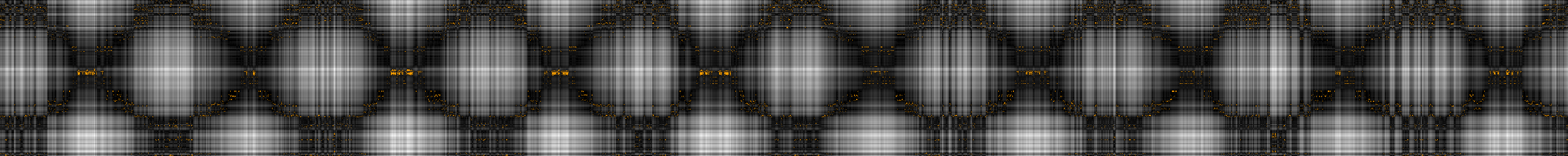
To work towards discovering whether this was indeed the case, I’ve plotted out the distance matrix for a 10 year by 10 year period. The plot is quite challenging to read, so settle in to stare at some weird patterns for a while.

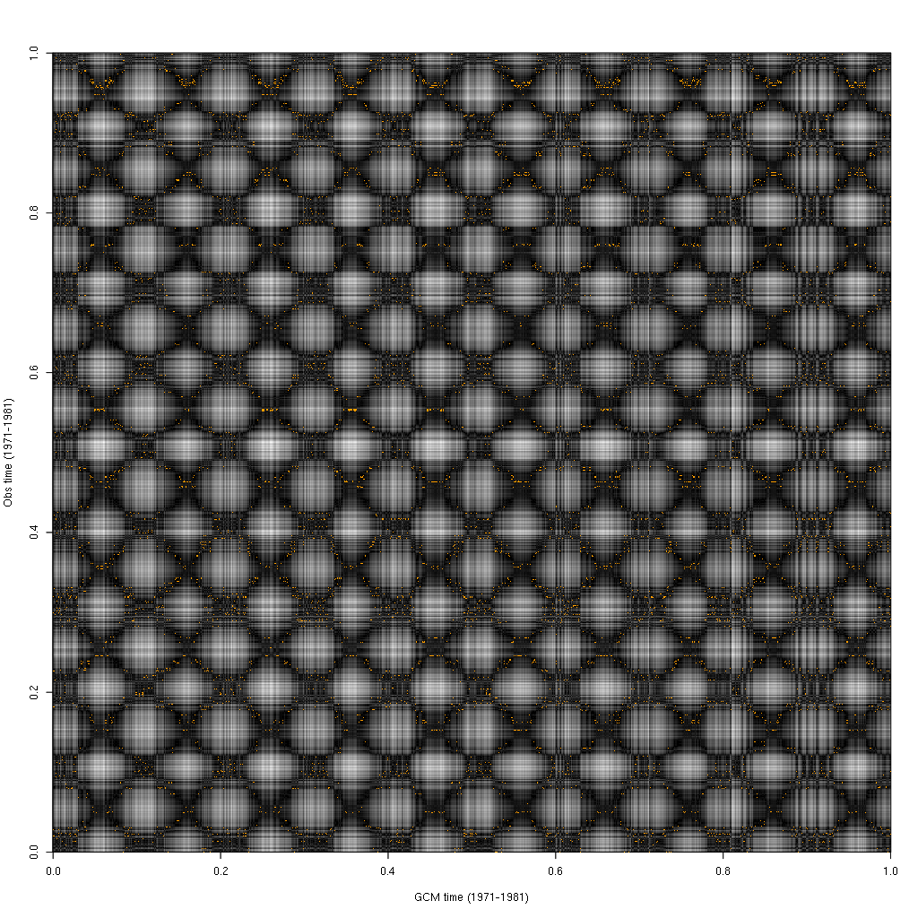BCCA distance matrix and selected timesteps

The x axis shows GCM time increasing from left to right while the y axis shows the observed time increasing from bottom to top. Pixels in the image are plotted in greyscale as the Euclidean distance from black to white. Time periods which are near to each other according to our distance function show as being darker, while those that are far apart show as being lighter. The top $k$ timesteps which are selected by BCCA are plotted as yellow points. The diagonal line for which the GCM time equals the observed time goes from the bottom left corner to the top right.

There are a number of features and patterns that might jump out. The first is the obvious lattice/hatching pattern. This is the correlation between similar seasons across both timeseries. Each of the smaller dark squares is a correlation between GCM winter and observed winter. The larger squares are the correlation between GCM summer and observed summer. The subtle diagonals that criss cross the plot are the correlations between fall/fall and spring/spring (for ascending diagonals) and fall/spring, spring/fall (for descending diagonals).

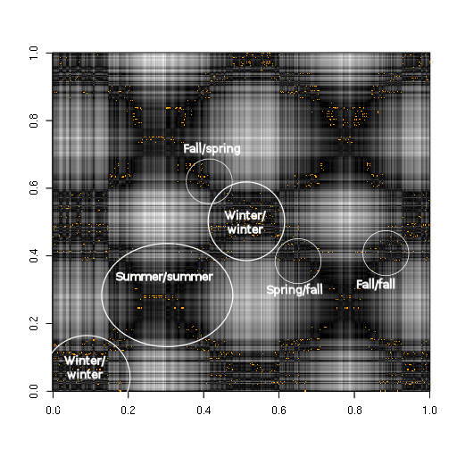Seasonality in the distance matrix Seasonal correlation shows up as large scale cross-hatching.

Within the large scale cross-hatching you can distinguish some smaller scale cross-hatching; vertical or horizontal likes that appear off color from their neighbors. These are unseasonably warm or unseasonably cold days that correlate better with the opposite season than the season in which they fall. For example, at about two-thirds ( $x=0.6$ ) of the way across the x axis you can see a series of lines that start out white in the winter, switch to dark in the summer, and pretty much swing back and forth out of phase to the top of the plot. These were some unseasonably warm days in the dead of winter. If you look follow the lines to the top looking for yellow dots (selected analogues), you’ll see that many analogues that were selected are either on the fringe of the observed period’s winter or completely apart from winter. None of this explains anything about BCCA’s performance, but I think that it’s helpful to explain graphically what the patterns mean in the base data.

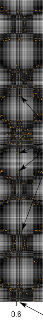BCCA distance matrix Unseasonable weather in the GCM shows up as vertical lines

One piece of evidence that we do have of distance correlation is the fact that some observation times are selected as analogues many times while other times are never selected. For example, look at the observed summer of 1976.

BCCA summer of '76 Days in the observed summer of 1976 (shown in the middle rows) were selected as analogues for wide number of GCM days

If you zoom in on the image you can see a few rows in the middle of the plot which have a large number of yellow dots clustered together. These clusters repeat multiple times from left to right. This is a particular chunk of observed days which are repeatedly selected as analogues year after year. These days are probably extremely close to each other, so any GCM day which matches one of them likely matches the rest. What can speed up this algorithm tremendously, is if we can find a way take advantage of similarities like these.

Limiting the analogue search space

The BCCA algorithm, as implemented, artificially limits the search space to a 90 day window surrounding the Julian day of the GCM time. Using the same plot type as above, we can visualize what this looks like.

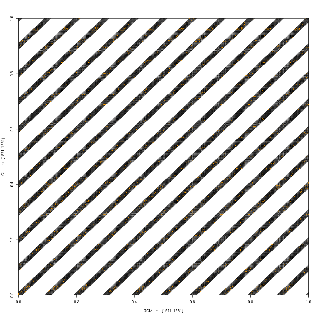Abbreviated BCCA distance matrix The BCCA distance matrix, as presently implemented.

I’m not sure whether this was intended to be an performance optimization with no side-effects, or whether the original authors specifically did not want analogues to be selected outside of a seasonal window.

I can say, however, the analogues would be selected from outside of the seasonal window if they could be. I’d love to know from the authors whether this would be desirable or not. If this was intended to be a performance optimization, it only scales the computation time by a constant factor ( $\frac{90}{365}$ ) and does not technically affect the computational complexity at all.

Conclusions

BCCA has a huge input size and a high computational complexity. This small glimpse is the first, to my knowledge, of any examinations of the internals of BCCA. I think that this shows that there are some obvious relationships amongst commonly selected analogues and some clear structure across which timesteps gets selected. How we leverage this structure to decrease the computational complexity of the algorithm remains elusive for now, but I’m confident that we can do so.

← Previous Archive Next →

blog comments powered by Disqus

Published

26 April 2016